Introduction to dominatR
Simon Lizarazo, Ethan Chen, Rajendra K C, Kevin Van Bortle
Source:vignettes/dominatR.Rmd
dominatR.RmdOverview
![]()
dominatR is a genomic data visualization package that
applies concepts drawn from physics - such as center of mass
from classical mechanics and Shannon’s entropy from statistical
mechanics - to effectively visualize features (e.g. genes) that are
present within a specific context or condition (e.g. tissue-specific
gene expression). dominatR is able to integrate
dataframes, matrices and
SummarizedExperiment objects, perform a number of common
genomic normalization methods, compute center of mass, entropy, and
categorical entropy values, and generate customizable plots that serve
to highlight context-relevant feature dominance. In all examples,
dominance visualization is linked to the coordinate spatial localization
of each data point, such that full feature dominance is projected at the
radial extreme.
dominatoR package functions can be subgrouped into the
following categories:
-
Normalization Functions: Contains basic normalization methods, such as:
cpm_normalizationminmax_normalizationquantile_normalizationrpkm_normalizationtpm_normalization
-
Calculation Functions: Contains feature calculation methods, such as:
centmassentropyQentropy
-
Visualization Functions: Contains three different visualization tools, ideal for assessing dominance in 2, 3 and N Dimension:
plot_ropeplot_triangleplot_circle
This vignette serves as a quick tutorial for using
dominatR. Further descriptions and examples of
customization and the additional features present in the package can be
explored in the companion articles.
Installation
To install this package, start R and enter
library(BiocManager)
BiocManager::install('dominatR')
Data normalization; computing and plotting feature dominance
The data included in this vignette can be found in the
airway dataset and the supplementary package
dominatRData
Normalization functions (e.g. quantile normalization)
Example 1: SummarizedExperiment object
data("airway")

se = quantile_normalization(airway, new_assay_name = 'quantile_norma')

head(se)
#> class: RangedSummarizedExperiment
#> dim: 6 8
#> metadata(1): ''
#> assays(2): counts quantile_norma
#> rownames(6): ENSG00000000003 ENSG00000000005 ... ENSG00000000460
#>   ENSG00000000938
#> rowData names(10): gene_id gene_name ... seq_coord_system symbol
#> colnames(8): SRR1039508 SRR1039509 ... SRR1039520 SRR1039521
#> colData names(9): SampleName cell ... Sample BioSample
head(assay(se, 'quantile_norma'))
#>                 SRR1039508 SRR1039509 SRR1039512 SRR1039513 SRR1039516
#> ENSG00000000003    690.875    504.750    773.875     613.75   1010.000
#> ENSG00000000005      0.000      0.000      0.000       0.00      0.000
#> ENSG00000000419    468.875    582.375    550.625     552.00    516.875
#> ENSG00000000457    257.375    241.375    225.250     254.00    213.125
#> ENSG00000000460     58.000     65.250     31.500      53.75     67.750
#> ENSG00000000938      0.000      0.000      1.250       0.00      0.375
#>                 SRR1039517 SRR1039520 SRR1039521
#> ENSG00000000003    757.375    878.250    608.750
#> ENSG00000000005      0.000      0.000      0.000
#> ENSG00000000419    582.125    467.500    541.625
#> ENSG00000000457    244.125    257.375    251.125
#> ENSG00000000460     48.375     79.875     66.000
#> ENSG00000000938      0.000      0.000      0.000
Example 2: dataframe object
data("atac_tissue_counts")

## selecting the numeric columns
norm = atac_tissue_counts[,8:26]

norm1 = quantile_normalization(norm)

head(norm1[,1:10])
#>           Heart     Spleen      Liver      Colon Adrenal.Gland       Lung
#> [1,]   11.26316   15.36842   13.00000   21.73684     13.789474   11.15789
#> [2,] 1369.78947 2997.36842 1679.36842 1422.52632   1486.421053 1549.94737
#> [3,]   17.78947   32.26316   57.89474   25.15789     21.789474   26.31579
#> [4,]   15.63158   14.78947   19.52632   22.78947      8.263158   15.26316
#> [5,]   17.78947   21.84211   20.84211   21.73684     15.000000   21.36842
#> [6,]   13.52632   18.57895   16.21053   17.89474     10.473684   13.10526
#>         Pancreas Gallbladder Urinary.Tract     Breast
#> [1,]    9.052632    11.89474      12.89474   14.26316
#> [2,] 1220.842105  1432.63158    1513.47368 1613.84211
#> [3,]   18.210526    16.84211      17.47368   19.42105
#> [4,]   14.894737    22.10526      14.68421   10.89474
#> [5,]   18.210526    20.00000      22.63158   16.52632
#> [6,]   10.631579    11.89474      25.10526   25.00000
Calculation functions (e.g. entropy)
Example 1: SummarizedExperiment object
se = entropy(se)

head(se)
#> class: RangedSummarizedExperiment
#> dim: 6 8
#> metadata(1): ''
#> assays(3): counts quantile_norma Entropy
#> rownames(6): ENSG00000000003 ENSG00000000005 ... ENSG00000000460
#>   ENSG00000000938
#> rowData names(11): gene_id gene_name ... symbol Entropy
#> colnames(8): SRR1039508 SRR1039509 ... SRR1039520 SRR1039521
#> colData names(9): SampleName cell ... Sample BioSample

### It creates a new column in the rowData dataframe
head(rowData(se))
#> DataFrame with 6 rows and 11 columns
#>                         gene_id   gene_name  entrezid   gene_biotype
#>                     <character> <character> <integer>    <character>
#> ENSG00000000003 ENSG00000000003      TSPAN6        NA protein_coding
#> ENSG00000000005 ENSG00000000005        TNMD        NA protein_coding
#> ENSG00000000419 ENSG00000000419        DPM1        NA protein_coding
#> ENSG00000000457 ENSG00000000457       SCYL3        NA protein_coding
#> ENSG00000000460 ENSG00000000460    C1orf112        NA protein_coding
#> ENSG00000000938 ENSG00000000938         FGR        NA protein_coding
#>                 gene_seq_start gene_seq_end    seq_name seq_strand
#>                      <integer>    <integer> <character>  <integer>
#> ENSG00000000003       99883667     99894988           X         -1
#> ENSG00000000005       99839799     99854882           X          1
#> ENSG00000000419       49551404     49575092          20         -1
#> ENSG00000000457      169818772    169863408           1         -1
#> ENSG00000000460      169631245    169823221           1          1
#> ENSG00000000938       27938575     27961788           1         -1
#>                 seq_coord_system      symbol   Entropy
#>                        <integer> <character> <numeric>
#> ENSG00000000003               NA      TSPAN6  2.917466
#> ENSG00000000005               NA        TNMD  0.000000
#> ENSG00000000419               NA        DPM1  2.961022
#> ENSG00000000457               NA       SCYL3  2.975398
#> ENSG00000000460               NA    C1orf112  2.955338
#> ENSG00000000938               NA         FGR  0.918296
Example 2: dataframe object
norm1 = entropy(norm)

### It creates a new column in the dataframe
head(norm1[,10:20])
#>       Breast Fallopian.Tube Psoas.Muscle  Vena.Cava Gastroesophageal.Sphincter
#> 1 0.06137184     0.06859206   0.02166065 0.06137184                 0.05415162
#> 2 0.02719477     0.05415596   0.08358637 0.05121959                 0.04261070
#> 3 0.05176471     0.05176471   0.02117647 0.05647059                 0.04705882
#> 4 0.04362416     0.07046980   0.03020134 0.05369128                 0.04362416
#> 5 0.04679803     0.11576355   0.01970443 0.06896552                 0.05665025
#> 6 0.07715134     0.04747774   0.02373887 0.05934718                 0.08902077
#>   Adipose.Tissue Sciatic.Nerve Ovary...Uterus    Stomach      Brain  Entropy
#> 1     0.04332130    0.06498195     0.05415162 0.05415162 0.12635379 4.090040
#> 2     0.03967433    0.06907137     0.07921519 0.02816243 0.03717174 4.137985
#> 3     0.04235294    0.06117647     0.05176471 0.04235294 0.06823529 4.116397
#> 4     0.05704698    0.04362416     0.04697987 0.06711409 0.10402685 4.123750
#> 5     0.04926108    0.04679803     0.03940887 0.04187192 0.11576355 4.071279
#> 6     0.05341246    0.05934718     0.05341246 0.05044510 0.11275964 4.062376
Visualization functions (2-, 3-, and N-dimensions)
All dominatR package functions are compatible with
SummarizedExperiment and data.frame objects.
This quick introduction will show examples using data.frame
objects. Each function produces a graphic and a data.frame
with the dominance results; setting the attribute
output_table = FALSE will restrict the dataframe from being
displayed. For more details and examples on usage and aesthetics
manipulation, refer to the articles in the visualization section.
Example 1: Two Dimensions with plot_rope()
plot_rope is useful to visualize feature dominance
between two variables. In this example the function is comparing
dominance over gene occupancy for RNA Polymerase II and RNA Polymerase
III. By default the function plots all data points, but users can adjust
entropy_range values to subset on observations within a
specified range.
data("rnapol_score")

data1 <- rnapol_score[,6:7]

plot_rope(
        data1,
        rope_color = 'white',
        pch = c(21, 21),
        push_text = 1.2,
        col = c('#7eb1d5', '#fa8451'),
        output_table = FALSE,
        rope_width = 1
)

title(main = 'Gene Occupancy RNA Pol II vs RNA Pol III',
        font.main = 1,
        cex = 0.5)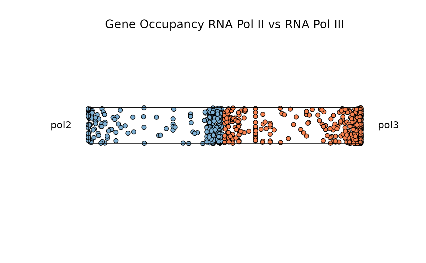
_____________________________
Below, let’s filter for genes with low entropy and high significance scores to visualize genes that are specifically occupied by either RNA Pol II or RNA Pol III
plot_rope(
        data1,
        rope_color = 'white',
        pch = c(21, 21),
        col = c('#7eb1d5', '#fa8451'),
        push_text = 1.2,
        output_table = FALSE,
        rope_width = 1,
        entropyrange = c(0, 0.5),
        maxvaluerange = c(1.3, Inf)
)


title(main = 'Gene Occupancy \n RNA Pol II vs RNA Pol III - Specific',
        font.main = 1,
        cex = 0.5)
_____________________________
Below, let’s filter for genes with high entropy and high significance scores to visualize genes that are specifically occupied by both RNA Pol II and RNA Pol III
plot_rope(
        data1,
        pch = c(21,21),
        push_text = 1.2,
        rope_color = 'white',
        col = c('#7eb1d5', '#fa8451'),
        output_table = FALSE,
        rope_width = 1,
        entropyrange = c(0.8, 1),
        maxvaluerange = c(1.3, Inf)
)

title(main = 'Gene Occupancy \n RNA Pol II vs RNA Pol III - Shared',
        font.main = 1,
        cex = 0.5)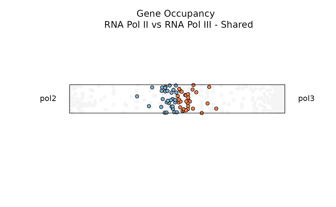
Example 2: Three Dimensions with plot_triangle()
plot_triange is useful to visualize feature dominance
between three variables. In this example, the function is comparing
dominance over gene occupancy for RNA Polymerase I, RNA Polymerase II
and RNA Polymerase III. By default the function plots every data point,
but users can again adjust the entropy_range attribute
values to subset on observations within a specified range.
data1 <- rnapol_score[,5:7]

plot_triangle(data1,
                output_table = FALSE,
                col = c('#ff80e3', '#7eb1d5', '#fa8451'),
                label = TRUE, pch = 21,
                push_text = 1.3)

title(main = 'Gene Occupancy \n Pol I vs Pol II vs Pol III',
        font.main = 1,
        cex = 0.5)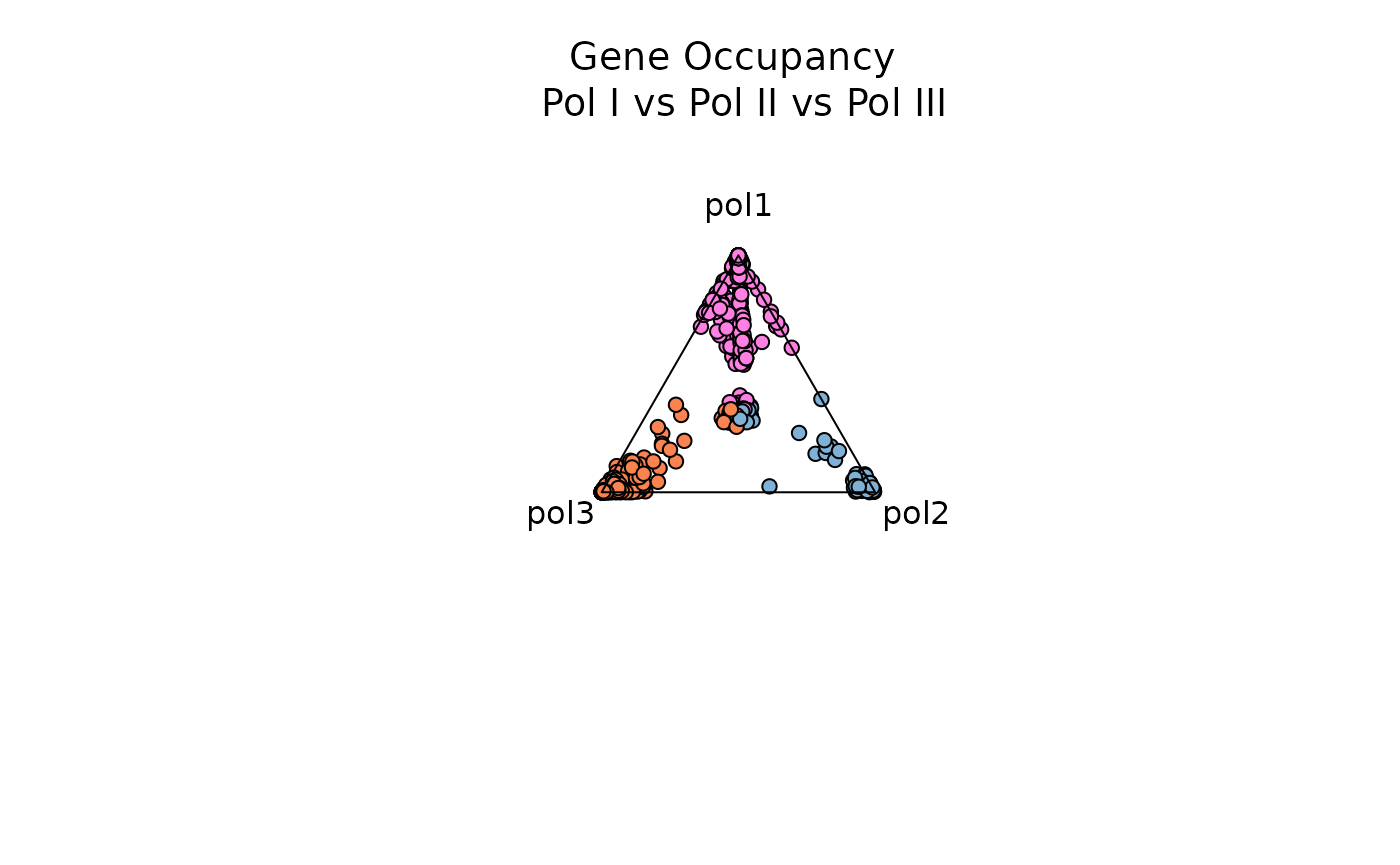
_____________________________
Below, let’s filter for genes with low entropy and high significance scores to visualize genes that are specifically occupied by either RNA Pol I, RNA Pol II, or RNA Pol III
data1 <- rnapol_score[,5:7]

plot_triangle(data1,
                output_table = FALSE,
                col = c('#ff80e3', '#7eb1d5', '#fa8451'),
                entropyrange = c(0,0.5),
                label = TRUE, pch = 21,
                push_text = 1.3)

title(main = 'Gene Occupancy \n Pol I vs Pol II vs Pol III - Specific',
        font.main = 1,
        cex = 0.5)
_____________________________
Below, let’s filter for genes with high entropy and high significance scores to visualize genes that are specifically occupied by all three RNA Pols or combinations of any 2 RNA Pols (e.g. RNA Pol I and RNA Pol II)
data1 <- rnapol_score[,5:7]

plot_triangle(data1,
                output_table = FALSE,
                col = c('#ff80e3', '#7eb1d5', '#fa8451'),
                entropyrange = c(1.5, Inf),
                label = TRUE, pch = 21,
                push_text = 1.3)

title(main = 'Gene Occupancy \n Pol I vs Pol II vs Pol III - Shared',
        font.main = 1,
        cex = 0.5)
Notice that as each data point gets closer to the center (and moving away from the vertices), the observation is characterized by higher entropy and is not dominated by a specific variable (in this case, by a specific RNA polymerase).
Example 3: N-Dimensions with plot_circle()
plot_circle is useful to visualize feature dominance
between N-Numbers of variables. In this example, the function is
comparing RNA-Pol III transcribed genes accessibility across tissues. By
default the function plots all the points, but the user can adjust
entropy_range values for subsetting specific type of
observations.
Briefly A total of P-1 (P = Number of Variables) circles are plotted and they represent degrees of dominance.
The outermost circle represents observations that are dominated only by one variable.
The second outermost circle represents observations that are dominated by two variables.
The innermost circle represents observations that are uniform across all variables.
data("atac_tissue_score")

### subsetting only a set of numerical columns
data1 = atac_tissue_score[,8:26]


plot_circle(data1,
            point_line_colors = rep('black', 19),
            magnituderange = c(1, Inf),
            n = 19,
            output_table = FALSE,
            point_size = 3) +
ggtitle('Pol III transcribed genes \n accessibility across tissues')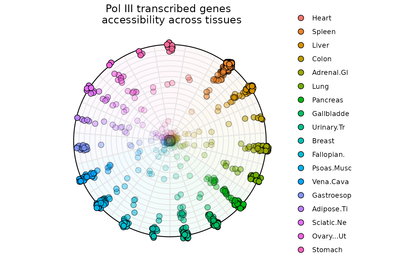
data("atac_tissue_score")


plot_circle(data1,
            point_line_colors = rep('black', 19),
            entropyrange = c(0,1),
            magnituderange = c(1, Inf),
            straight_points = FALSE,
            n = 19,
            output_table = FALSE,
            point_size = 3) +
ggtitle('Pol III transcribed genes \n accessibility across tissues - Unique')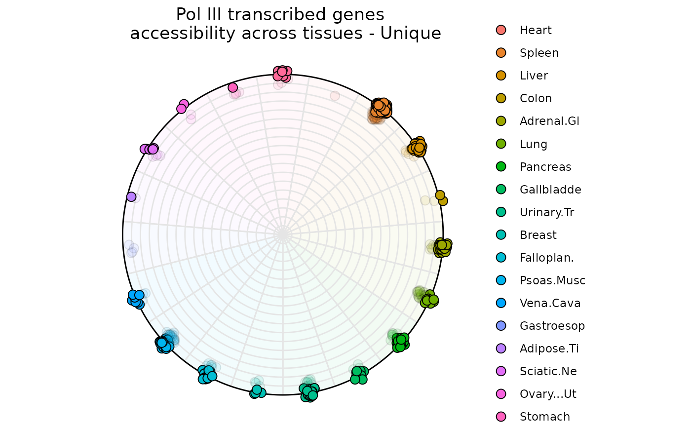
data("atac_tissue_score")

plot_circle(data1,
            point_line_colors = rep('black', 19),
            entropyrange = c(4, Inf),
            magnituderange = c(1, Inf),
            n = 19,
            output_table = FALSE,
            point_size = 3) +
ggtitle('Pol III transcribed genes \n accessibility across tissues - Shared')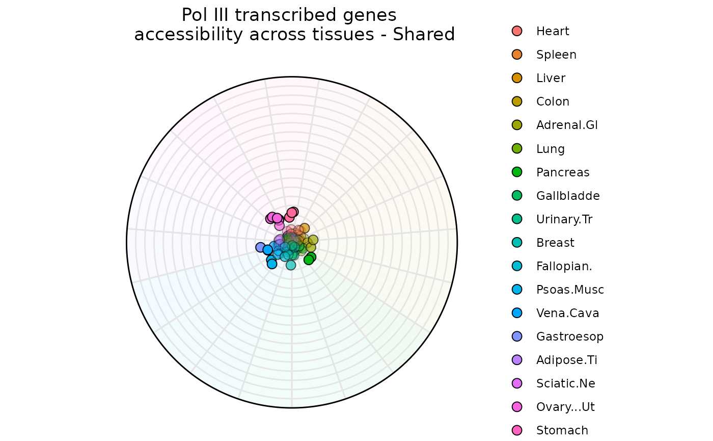
Session Info
#> R version 4.6.0 (2026-04-24)
#> Platform: x86_64-pc-linux-gnu
#> Running under: Ubuntu 24.04.4 LTS
#>
#> Matrix products: default
#> BLAS:   /usr/lib/x86_64-linux-gnu/openblas-pthread/libblas.so.3
#> LAPACK: /usr/lib/x86_64-linux-gnu/openblas-pthread/libopenblasp-r0.3.26.so;  LAPACK version 3.12.0
#>
#> locale:
#>  [1] LC_CTYPE=C.UTF-8       LC_NUMERIC=C           LC_TIME=C.UTF-8
#>  [4] LC_COLLATE=C.UTF-8     LC_MONETARY=C.UTF-8    LC_MESSAGES=C.UTF-8
#>  [7] LC_PAPER=C.UTF-8       LC_NAME=C              LC_ADDRESS=C
#> [10] LC_TELEPHONE=C         LC_MEASUREMENT=C.UTF-8 LC_IDENTIFICATION=C
#>
#> time zone: UTC
#> tzcode source: system (glibc)
#>
#> attached base packages:
#> [1] stats4    stats     graphics  grDevices utils     datasets  methods
#> [8] base
#>
#> other attached packages:
#>  [1] ggplot2_4.0.3               airway_1.31.0
#>  [3] SummarizedExperiment_1.41.1 Biobase_2.71.0
#>  [5] GenomicRanges_1.63.2        Seqinfo_1.1.0
#>  [7] IRanges_2.45.0              S4Vectors_0.49.3
#>  [9] BiocGenerics_0.57.1         generics_0.1.4
#> [11] MatrixGenerics_1.23.0       matrixStats_1.5.0
#> [13] dominatRData_0.99.1         dominatR_1.1.0
#> [15] knitr_1.51
#>
#> loaded via a namespace (and not attached):
#>  [1] sass_0.4.10         SparseArray_1.11.13 lattice_0.22-9
#>  [4] digest_0.6.39       magrittr_2.0.5      RColorBrewer_1.1-3
#>  [7] evaluate_1.0.5      grid_4.6.0          fastmap_1.2.0
#> [10] jsonlite_2.0.0      Matrix_1.7-5        ggnewscale_0.5.2
#> [13] scales_1.4.0        tweenr_2.0.3        textshaping_1.0.5
#> [16] jquerylib_0.1.4     abind_1.4-8         cli_3.6.6
#> [19] rlang_1.2.0         polyclip_1.10-7     XVector_0.51.0
#> [22] withr_3.0.2         cachem_1.1.0        DelayedArray_0.37.1
#> [25] yaml_2.3.12         S4Arrays_1.11.1     tools_4.6.0
#> [28] dplyr_1.2.1         vctrs_0.7.3         R6_2.6.1
#> [31] lifecycle_1.0.5     fs_2.1.0            MASS_7.3-65
#> [34] ragg_1.5.2          pkgconfig_2.0.3     desc_1.4.3
#> [37] pkgdown_2.2.0       bslib_0.10.0        pillar_1.11.1
#> [40] gtable_0.3.6        glue_1.8.1          ggforce_0.5.0
#> [43] systemfonts_1.3.2   xfun_0.57           tibble_3.3.1
#> [46] tidyselect_1.2.1    farver_2.1.2        htmltools_0.5.9
#> [49] labeling_0.4.3      rmarkdown_2.31      compiler_4.6.0
#> [52] S7_0.2.2            geomtextpath_0.2.0